(Latest Revision: Fri Mar 03 2023)
[2023/03/03: more boldface highlights]
[2023/02/26: boldface highlights]
[2023/02/26: minor rewording]
[2022/02/25: fixed a typo]
[2021/02/19: repositioned a figure]
[2019/06/03: minor edits]
[2019/06/01: added more figures]
[2019/03/21: format changes]
[2019/02/25: previous updates]
Chapter Five -- CPU Scheduling -- Lecture Notes
This chapter covers ideas about scheduling in general purpose computing systems, and also in real-time systems. Nowadays, a modern operating system schedules kernel-threads.
However, this text and other computer science literature still use the terms "job scheduling"
and "process scheduling" as names for such OS scheduling activity.
5.0 Objectives
Describe various CPU scheduling algorithms. (yes)
Assess CPU scheduling algorithms based on scheduling criteria.
(We discuss advantages and disadvantages)
Explain the issues related to multiprocessor and multicore scheduling. (yes)
Describe various real-time scheduling algorithms. (briefly)
Describe the scheduling algorithms used in the Windows, Linux, and
Solaris operating systems. (briefly)
Apply modeling and simulations - ways to evaluate CPU scheduling algorithms.
(brief discussion of each of a list of approaches)
Design a program that implements several different CPU scheduling
algorithms. (no)
5.1 Basic Concepts
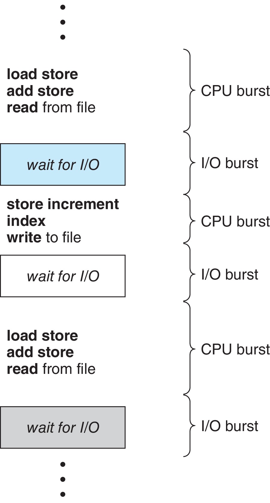
5.1.1 CPU-I/O Burst Cycle
Figure 5.1: CPU-I/O Burst Cycle
Generally, processes alternate between CPU bursts and
I/O bursts.
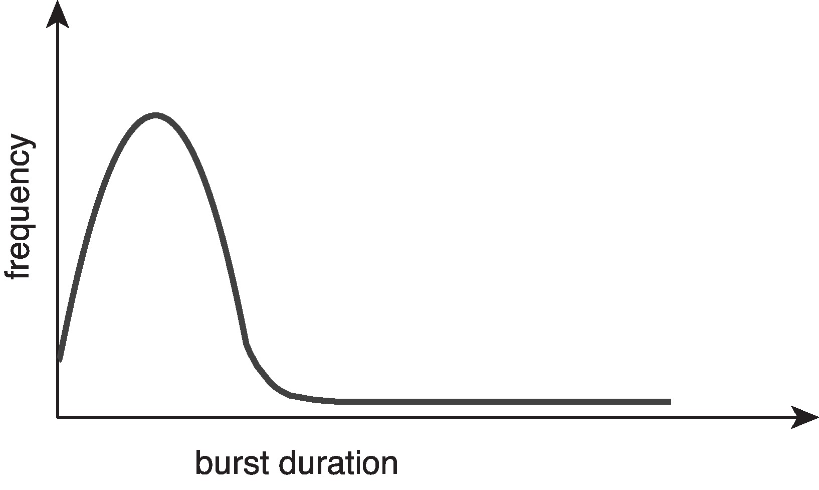
For a typical process, when we make a graph of the frequency
of CPU bursts versus the duration, we see a
hyperexponential shape. Basically it means there are
lots of short bursts and few long ones.
Figure 5.2: Histogram of CPU-burst durations
5.1.2 CPU Scheduler
The job of the short-term scheduler of the OS is to choose
the next job from the ready queue to be allowed to run in the CPU.
Conceptually, the data structure in the ready queue is a process
control block (PCB). (Quite likely, it's a thread control
block, but this is one of those situation where we use "traditional
names.") As you may know, the ready queue may NOT be structured as
a first-in, first-out queue.
5.1.3 Preemptive and Nonpreemptive Scheduling
Sometimes the current process, P, in the CPU is removed from the CPU
by an interrupt or trap, but it remains ready to run and goes
immediately back into the ready queue. If, under those
circumstances, the short-term scheduler decides to run a process
other than P next, then we say P has been preempted. A
scheduler capable of preempting is called a preemptive
scheduler.
In modern computing systems it is very common to allow preemption.
That makes the systems more responsive to interactive users, and
more supportive of processes when they urgently need to execute
in a CPU.
However, there is danger that processes that are
preempted will leave data or other resources in inconsistent
states. For example, suppose the process P is preempted while it
is inserting an element into a queue. In other words, the insert
operation is discontinued when it is only half done.
If M is the next process to execute, and if M attempts to perform
an operation on the same queue, then quite likely the queue structure
will be corrupted.
This kind of problem is called a race condition.
It happens when two or more operations are attempted
concurrently, and the correctness of the outcome depends
on the particular order in which the operations are performed.
People have to design preemptive
systems carefully so that race conditions and other
synchronization problems don't cause damage.
5.1.4 Dispatcher
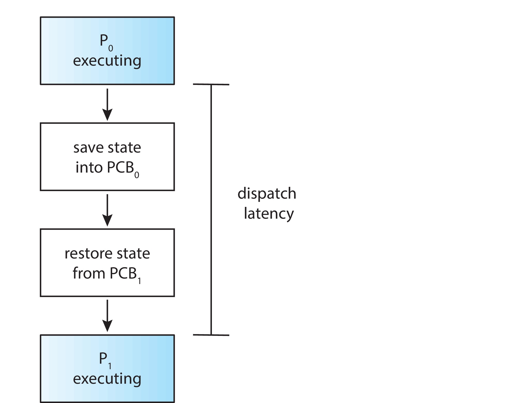
Figure 5.3: The role of the dispatcher
& dispatch latency
The dispatcher is the part of the OS that actually puts a
process in the CPU. After the scheduler selects the next process
to run in the CPU, the scheduler calls the dispatcher. The dispatcher
performs the data movement associated with context switching,
switches to user mode, and jumps to the requisite
instruction within the user process. It is very important to
design the code of the dispatcher so that it runs as
quickly as possible. The dispatcher is a performance bottleneck
on many systems. The time the dispatcher uses up is called
the dispatch latency.
5.2 Scheduling Criteria
The scheduler's scheduling algorithm can affect
all these performance measures:
CPU utilization
== (time CPU runs 'useful' code) / (total elapsed time)
CPU utilization is often multiplied by 100 and
expressed as a percentage, like 84%, instead of 0.84.
throughput == number of jobs completed per unit time
turnaround time == the time from submission to completion
wait time == time spent in the ready queue Beware of confusion here: It may go against your
intuition. "Wait time" does NOT include any of the time
spent while the process is in the waiting state - such as
waiting for I/O.
response time == time from submission
to start of first response
Typical goals of short-term scheduling are high CPU utilization, high throughput,
short turnaround time, short wait time, and short response time.
Generally system designers also want the measures of
performance above to have low variance.
5.3 Scheduling Algorithms
5.3.1 First-Come, First-Served Scheduling
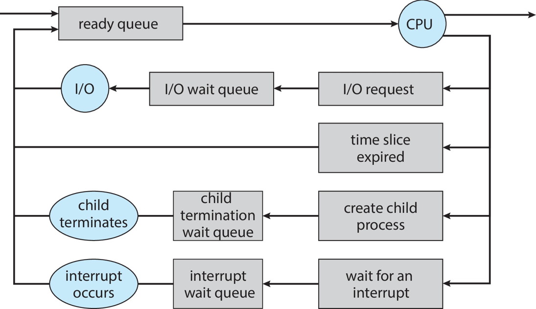
Figure 3.5: Queueing-diagram Representation of Process
Scheduling When the ready queue is a
first-in, first-out (FIFO) queue,
the resulting scheduling algorithm is FCFS.
Advantage: FCFS is easily understood and implemented.
Disadvantages:
There can be long average wait time.
FCFS is non-preemptive, which can lead to poor response time.
FCFS is subject to the "convoy effect" causing
low utilization of CPUs and I/O channels
because groups of I/O-bound processes get stuck in
queues behind CPU-bound processes.
5.3.2 Shortest-Job-First Scheduling
Advantage: Pure SJF has a "minimum average wait time"
optimality property.
Disadvantage:Starvation of long jobs is possible.
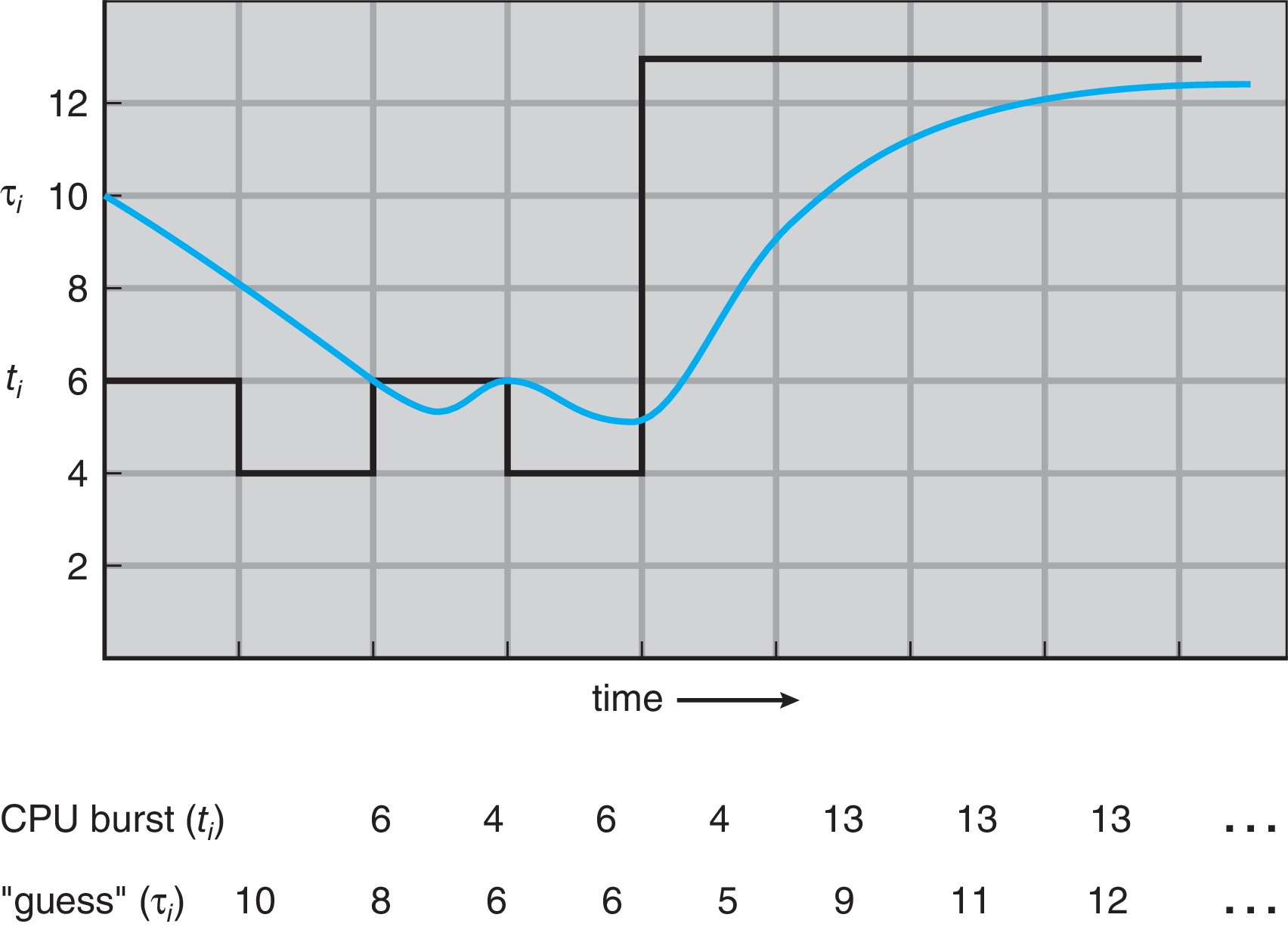
Detail: SJF can't be implemented perfectly at the level of
short-term scheduling. Instead the scheduler employs an estimate
of the length of the next burst Figure 5.4: Prediction of the length of the next CPU burst
Detail:SJF may be preemptive or non-preemptive.
If preemptive, when a new job N arrives in the ready queue,
and N is shorter than the remainder of the current job K
in the CPU, the scheduler must replace K with N as soon as possible.
Starvation:
(a.k.a. indefinite postponement)
If new, short jobs keep arriving frequently enough, a long job may
wait indefinitely in the ready queue, because there is always a
shorter job waiting there, and the scheduler will execute the
shorter job.
This phenomenon is similar to what happens if you go to the
emergency room with a sore throat. You will be served if and when
there is no one there with a more urgent need. After all the people
who were there when you arrived are served, you may still have to
wait longer because more people who need care more
urgently than you may have arrived in the meantime .
There is no limit to the number of people who will be
served before you are served. There is no means of knowing
whether you will be served eventually.
5.3.3 Round-Robin Scheduling
Advantage: RR helps time-sharing systems have short
response time.
Disadvantage: High average wait times Disadvantage: Time lost context-switching
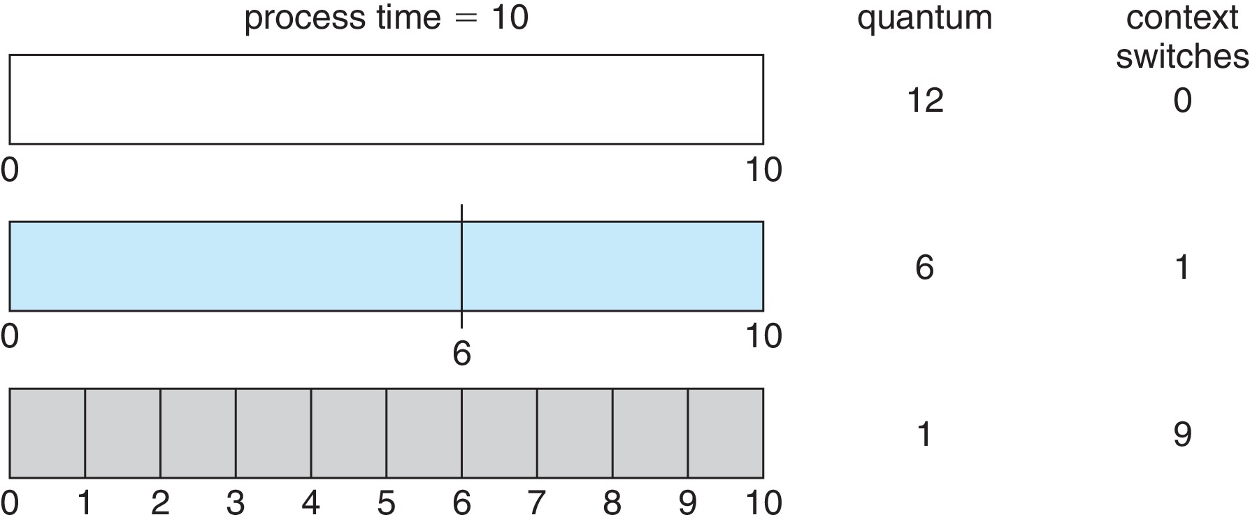
Detail: RR uses a circular queue and a time-slice (quantum). Detail: RR is preemptive. Detail: To avoid excessive overhead the quantum
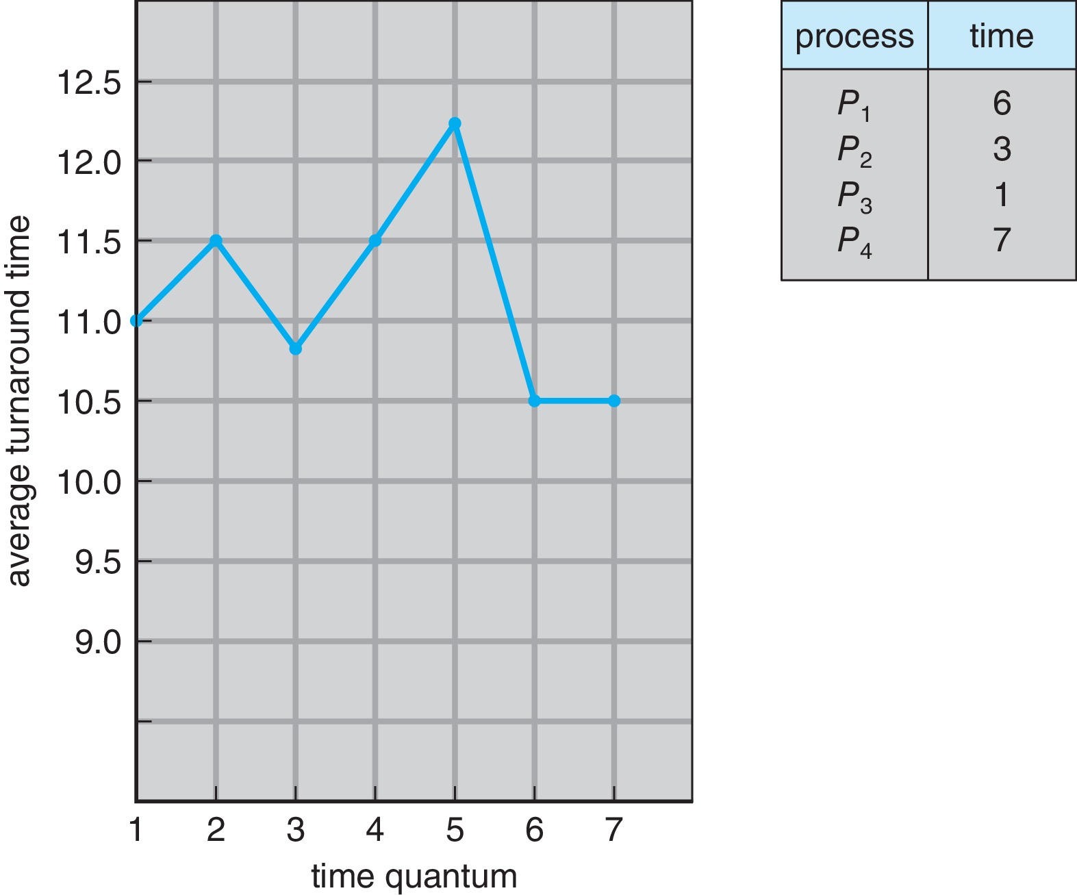
must be much larger than the context-switch time. Detail: To get low turnaround times the quantum
must be larger than the average CPU burst time. Detail: On the other hand the quantum has to be small
enough to produce good response time. Heuristic: 80% of the CPU bursts should be shorter than
the quantum. Quantum Range:Typically between 10 ms and 100 ms on general-purpose systems.
Figure 5.5: How a smaller time quantum increases context switchesFigure 5.6: How turnaround time varies with time quantum
5.3.4 Priority Scheduling
* Disadvantage: HPJF can lead to starvation.
(SJF is a form of HPJF.)
* Detail: Aging used in conjunction with HPJF can avert starvation.
Aging is the elevation of the priority of processes
that have not received CPU time.
* Detail: HPJF can be preemptive or non-preemptive.
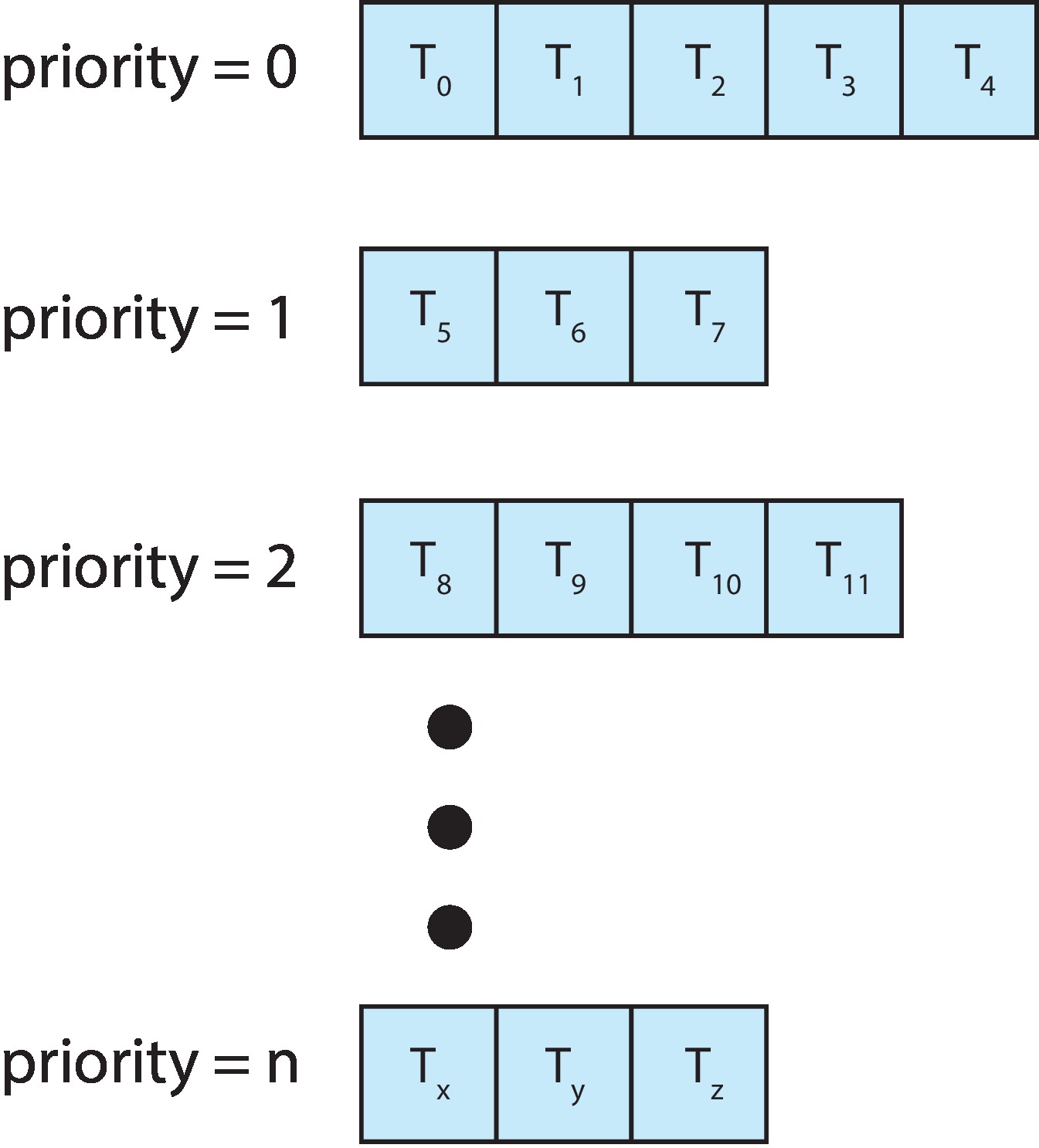
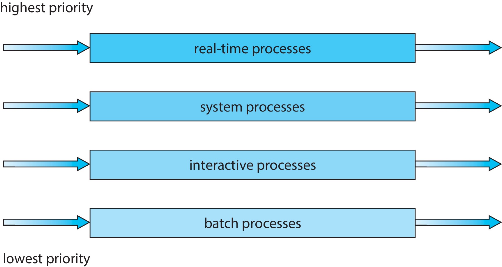
5.3.5 Multilevel Queue Scheduling
Figure 5.7: Separate queues for each priority
Figure 5.8: Multilevel queue scheduling
The method of scheduling may be based on
having a separate ready-queue for each process priority, or
dividing processes into several types and having
a separate ready-queue for each process type
(e.g. foreground processes, background, system,
interactive editing, ...)
Each queue can have a different scheduling algorithm,
say, tailored to the type of process.
The multilevel queue design must include an algorithm that
decides which queue to service, and when. This algorithm might
implement strict priorities among queues. In that case the
scheduler would always service the highest priority queue that is
not empty. Another option is to do time-slicing among the queues.
In other words, jump from queue to queue, running jobs from each
one for a short time quantum.
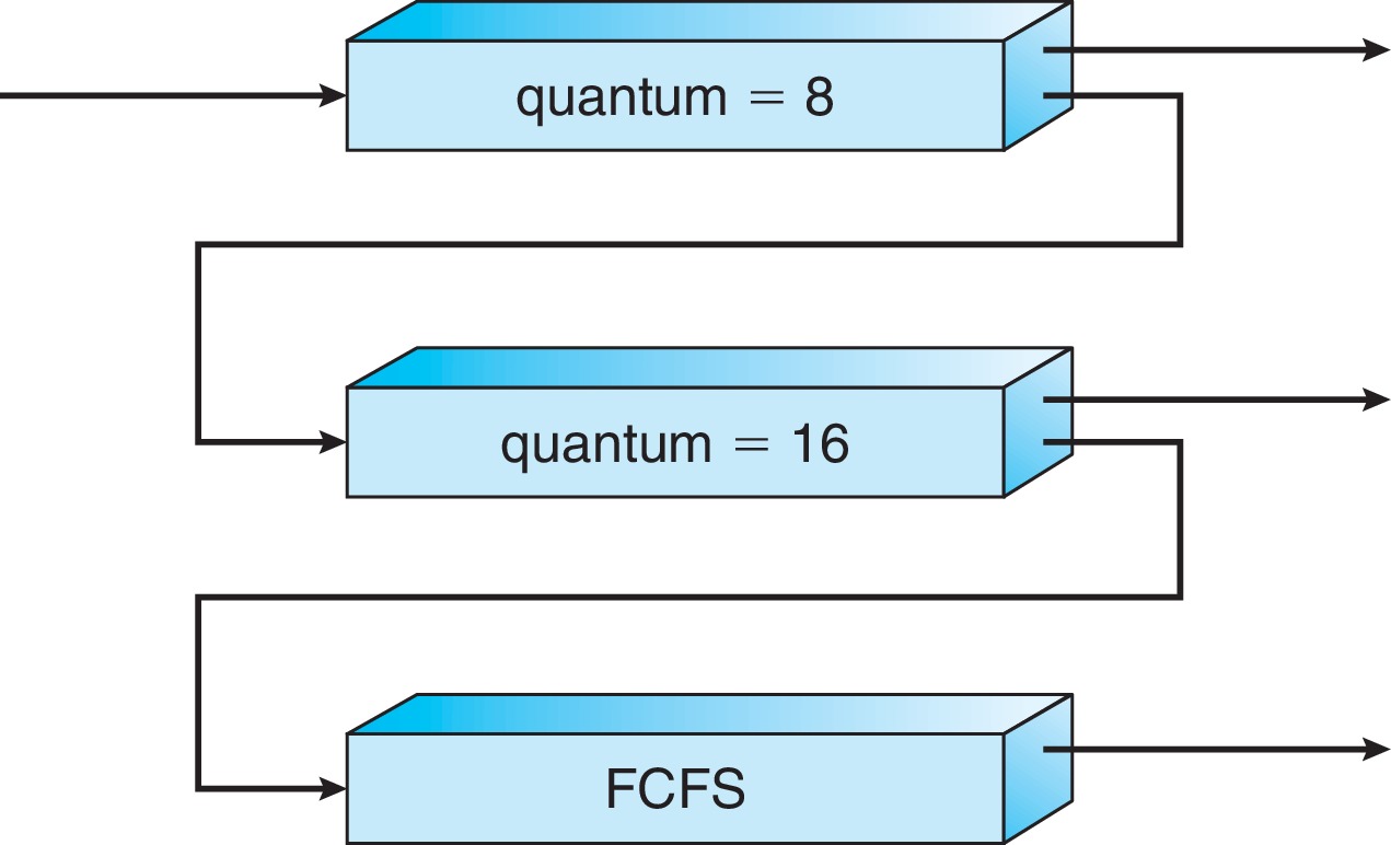
5.3.6 Multilevel Feedback Queue Scheduling
Figure 5.9: Multilevel feedback queues
In the words of the text, "this is the most general CPU-scheduling
algorithm," allowing designers to configure it to match a large
range of design goals. However it makes the design process quite
complicated.
A main idea is to put jobs in queues based on recent CPU usage.Allow migration from queue to queue. Processes that "over-use" CPU
time move to a lower priority queue, and processes that become
"starved" for CPU time move to a higher priority queue.
There may be other reasons for moving processes from one queue to another.
5.4 Thread Scheduling
I won't cover this section in lecture or ask anything about it on tests. Basically it compares and contrasts scheduling issues of user-level threads
versus kernel-level threads. It also discusses Pthreads API functions
that, under some conditions, allow a programmer to choose between, for example,
the many-to-many model and the one-to-one model.
5.4.1 Contention Scope
5.4.2 Pthread Scheduling
5.5 Multiprocessor Scheduling
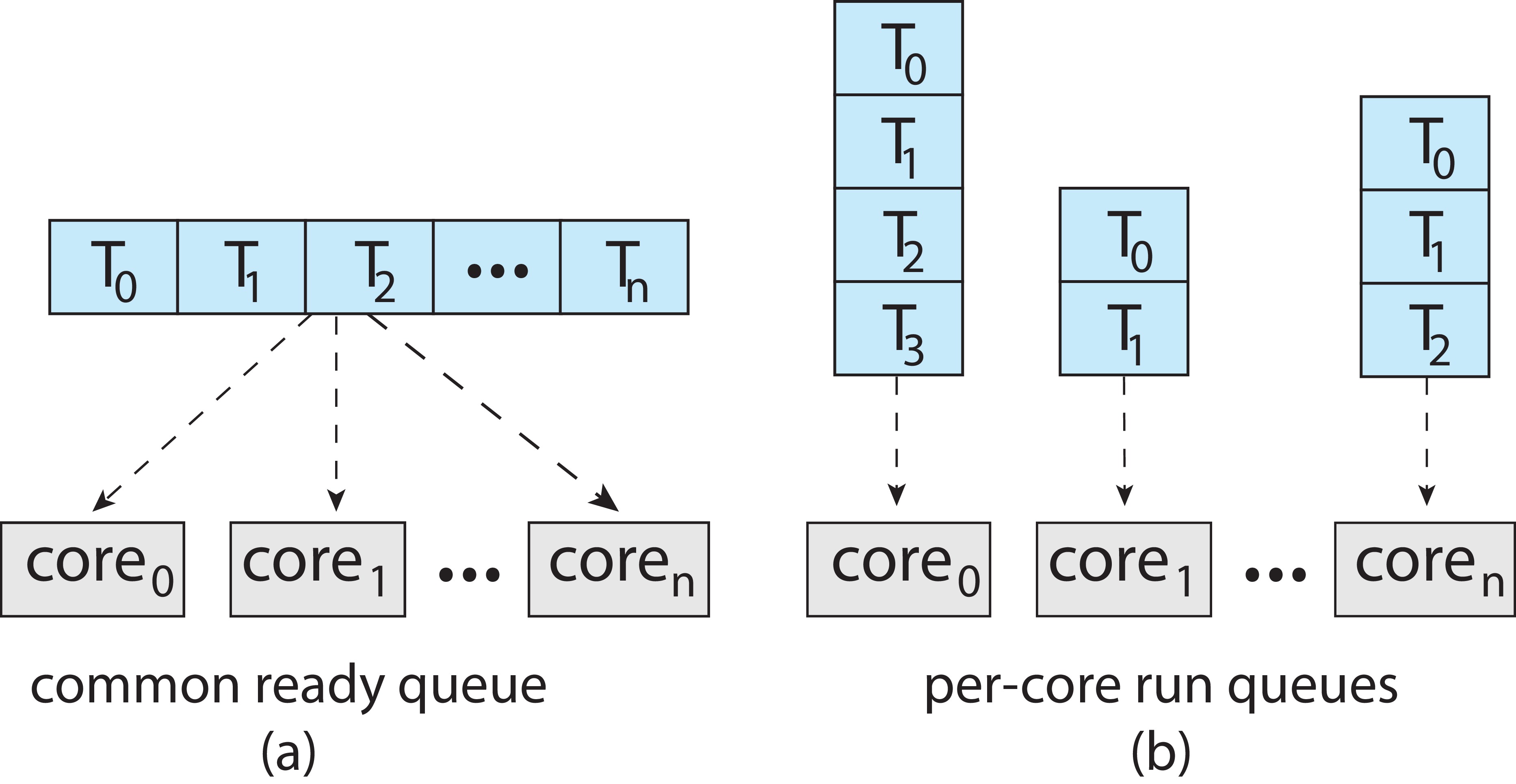
5.5.1 Approaches to Multiple-Processor Scheduling
Figure 5.11: Approaches to Multiple-Processor SchedulingAsymmetric Multiprocessing (AMP) is a possibility: All OS
code runs on just one of the processors,
and so only one process at a time has
access to system data structures. This avoids synchronization
problems.
Virtually all modern operating systems supportSymmetric Multiprocessing (SMP)
- operating system code can run on any processor.
There is a separate scheduler for each
processor.
SMP can be used in conjunction with either a common ready queue or
separate ready queues for each processor. (See figure 5.11.)
Access to a common ready queue has to be programmed carefully
(synchronization problem).
On the other hand, load balancing can be problematic if there is a
separate ready queue for each processor. What if some queues are
empty and others are full?
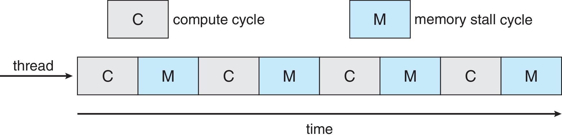
5.5.2 Multicore Processors
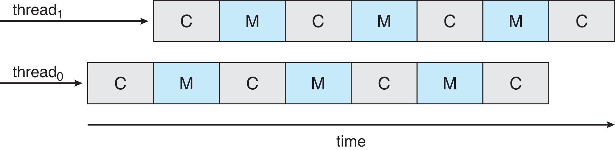
Figure 5.12: Memory StallFigure 5.13: Multithreaded Multicore SystemFigure 5.14: Chip Multithreading
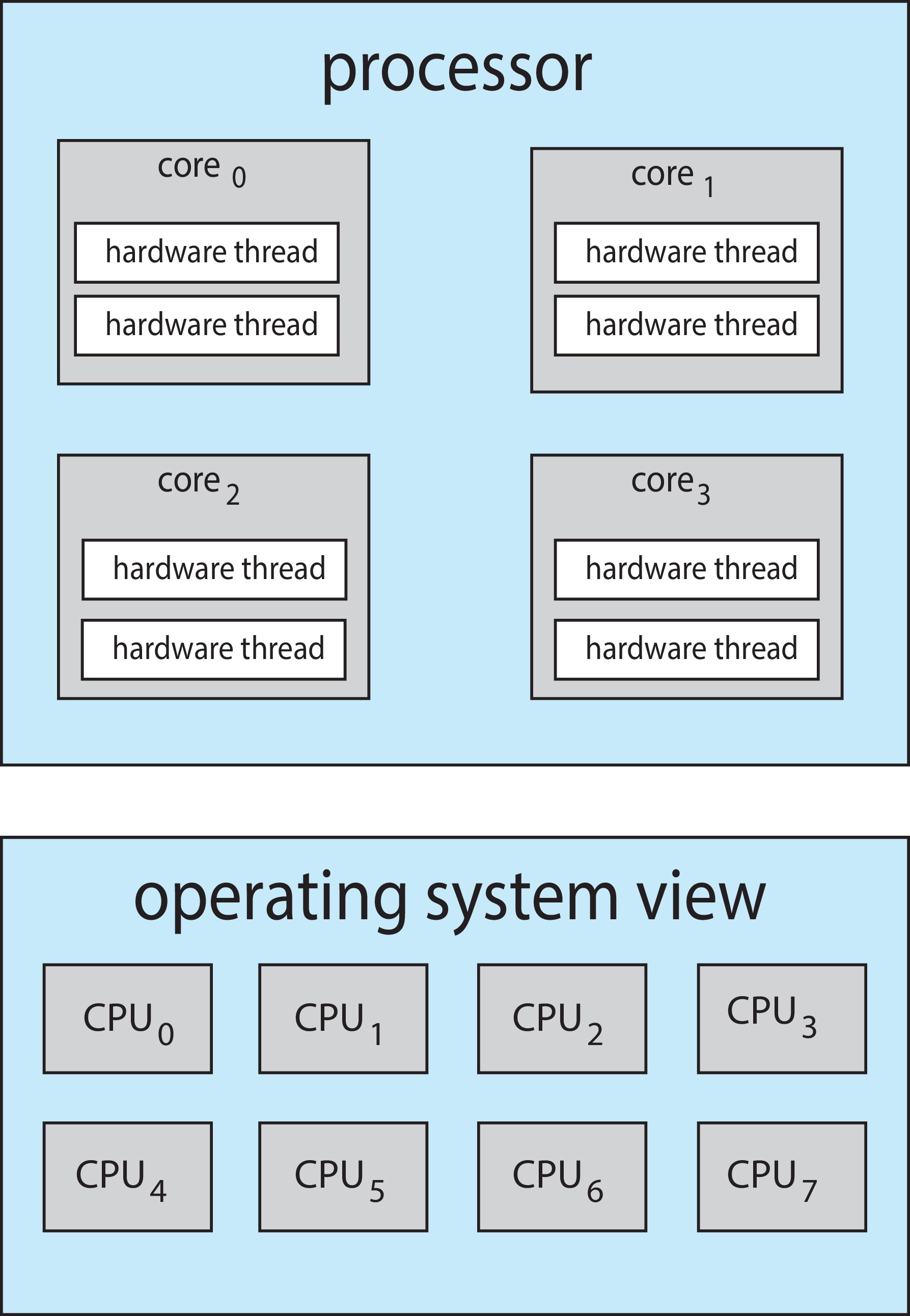
Multicore processors are basically multiprocessors on a single chip.
A core may implement two or more logical processors by supporting
the compute cycle of one thread during the memory stall cycle(s) of
the other(s).
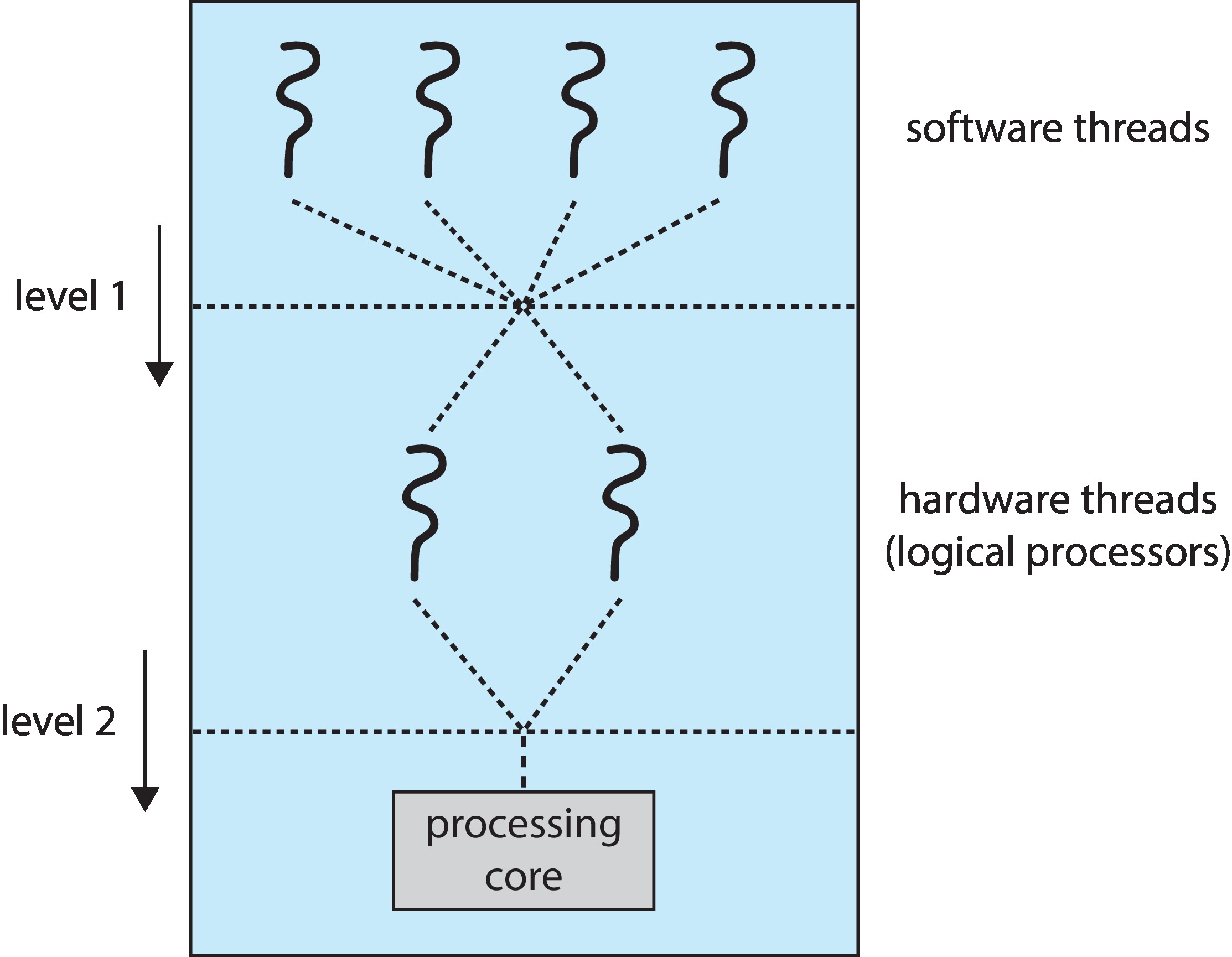
Figure 5.15: Two levels of scheduling
This means that one level of scheduling is done by the hardware of
the cores when they select among the threads assigned to them.
5.5.3 Load Balancing
When each processor has a separate ready queue, there can be an
imbalance in the numbers and/or kinds of jobs in the queues. Push
and pull migration are standard approaches to load balancing:
With push migration, a system process periodically
checks ready queues and moves processes to different queues,
if need be. If you are waiting for a cashier at a large store
and a floorwalker directs you to another queue, that is similar
to push migration.
With pull migration, OS code running on each
processor X notices when X has little work to do,
and tries to take jobs from other ready queues. When
you are waiting for one checker at a food market, and
another checker says "I can help you over here," that
is similar to pull migration.
5.5.4 Processor Affinity
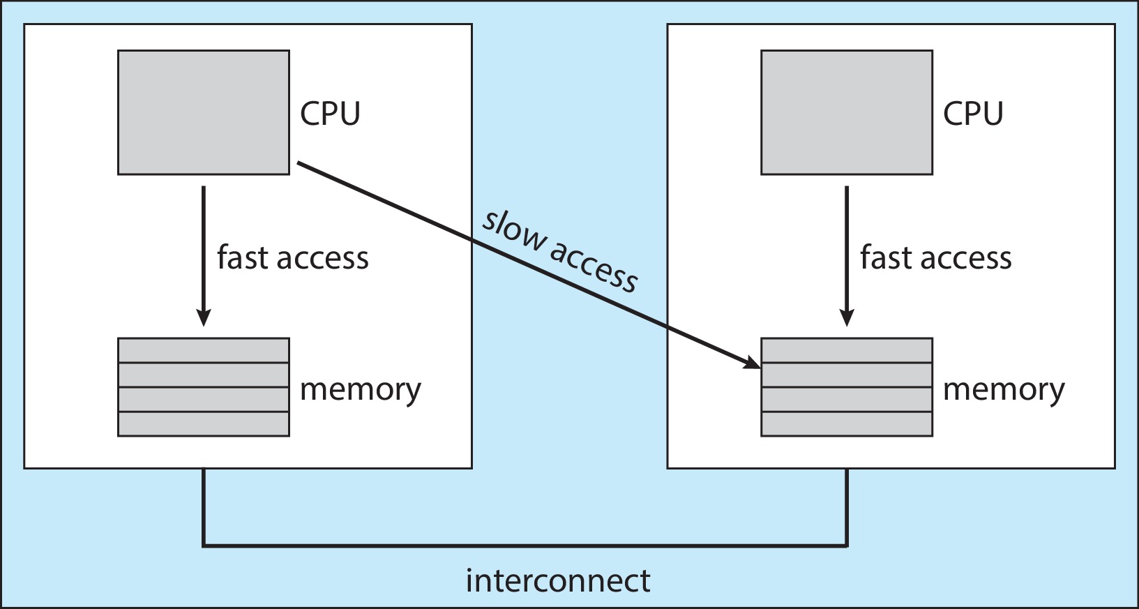
Figure 5.16: NUMA and CPU schedulingProcessor Affinity Problem: If a process migrates from one CPU
to another, the old instruction and address caches become invalid,
and it will take time for caches on the new CPU to become 'populated'.
For this reason, OS designers may build the short-term scheduler
to treat processes as having affinity for the CPU on which
they have been executing most recently.
The idea of soft processor affinity is for the
scheduler to give
priority to putting the process on its 'home' CPU, but not to make
doing so an absolute requirement. With
hard processor affinity, there's little or
no flexibility
to allow a process to migrate to a different CPU.
Another factor is architectures with non-uniform memory access
(NUMA) -- e.g. when there are multiple units with integrated CPU
and memory. Here it is advantageous for the scheduler and memory
allocator to cooperate to keep a process running on the CPU
that is 'close' to the memory in which it is resident.
Note that load balancing tends to work counter to the idea of
processor affinity.
5.5.5 Heterogeneous Multiprocessing
In a heterogeneous multiprocessor (HMP),
the processors may not
all be essentially equivalent to each other.
An example is the big.LITTLE architecture supported by some
Advanced Risc Machines (ARM) processors. There are
high-performance but power-hungry big cores,
and energy-efficient but lower-performance little cores.
A CPU scheduler, particularly on a mobile device,
can take advantage of a system like that. For
example, it may schedule long-running low-demand background
processes on little cores, and performance-hungry applications
that don't run for long on big cores.
5.6 Real-Time CPU Scheduling
DEFINITION: Soft real-time systems guarantees only to give high
priority to certain processes with real-time requirements.
DEFINITION: Hard real-time systems guarantee that certain processes
will execute within their real-time constraints.
5.6.1 Minimizing Latency
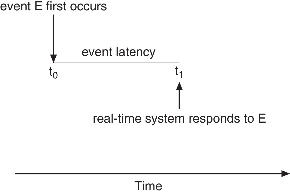
Figure 5.17: Event Latency
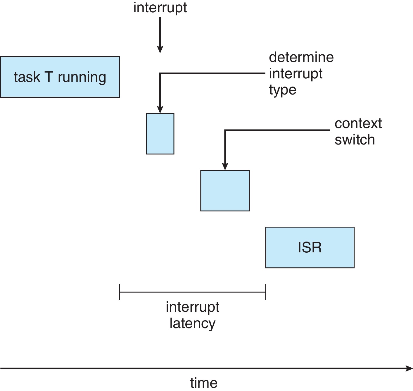
Figure 5.18: Interrupt Latency
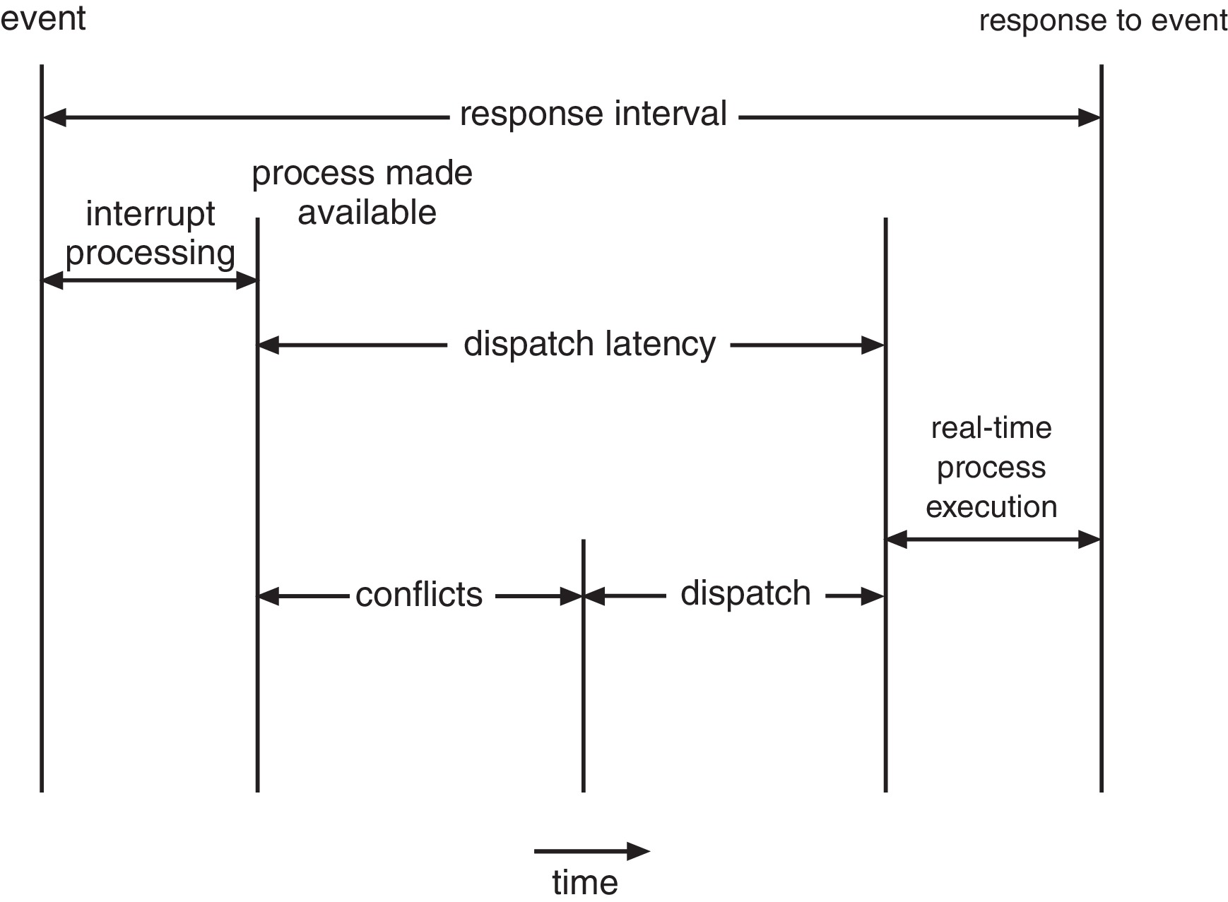
Figure 5.19: Dispatch Latency
In order to assure that deadlines are met, a hard real-time
system must enforce a bound on interrupt latency, the
elapsed time between when an interrupt arrives at a CPU and
when the service routine for the interrupt starts execution.
Other ways to help assure
that deadlines can be met:
Require that interrupts be disabled only for very
short periods of time.
Implement a dispatcher that performs very fast
context switches.
Allow preemption of processes, so that high priority
processes can be dispatched without delay.
Create means for low-priority processes to
quickly release resources needed by a high-priority
(real-time) process.
5.6.2 Priority-Based Scheduling
The text considers periodic hard real-time processes.
These
processes require the CPU at constant intervals (periods).
An example, found
here
is "a video decompressor may have to run 30 times
per second at 33.3 millisecond intervals."
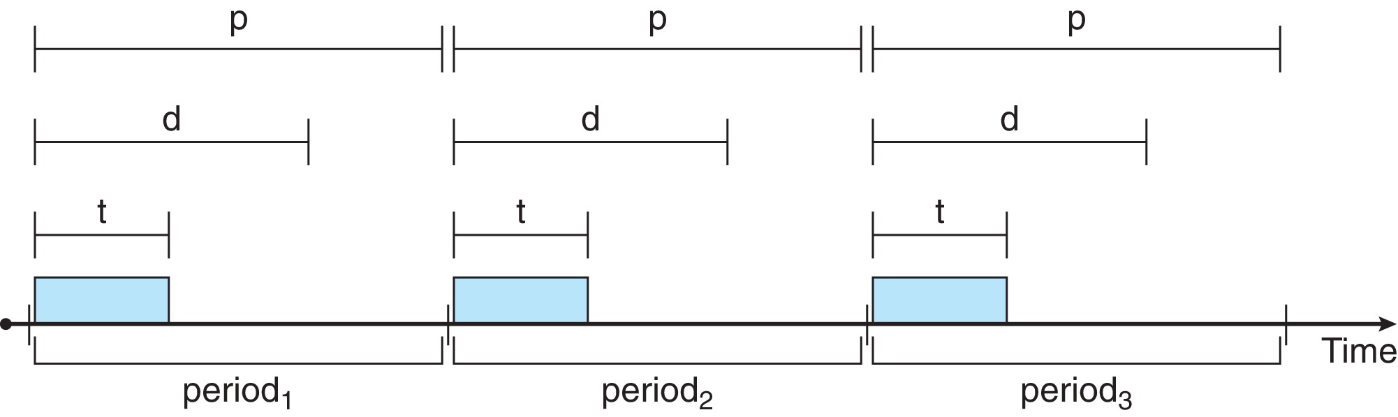
Besides the period p, two other constants are associated
with a periodic process, the time t required to complete
the task, and the deadline d. We assume the relation
0 ≤ t ≤ d ≤ p
Figure 5.20: Periodic tasks
One of the jobs of the scheduler in a hard real-time system
is to examine the characteristics of each periodic process,
and determine whether it (the scheduler) can guarantee
that the deadline(s) of the process will always be met.
If so, the scheduler admits the process.
If not, the scheduler rejects the process.
5.6.3 Rate-Monotonic Scheduling
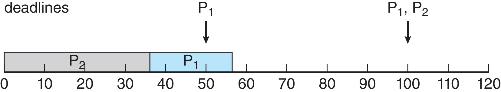
Figure 5.21: Scheduling of tasks when P2 has a higher priority than P1
Rate-monotonic scheduling utilizes static priorities
and preemption.
Periodic processes with shorter periods have priority over
periodic processes with longer periods.
With this scheduling discipline, a set of periodic processes
have the 'best chance' of meeting all deadlines. In
other words, if rate-monotonic scheduling does not allow
the processes to always meet their deadlines, then no other
algorithm that assigns static priorities can do so.
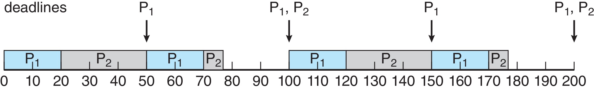
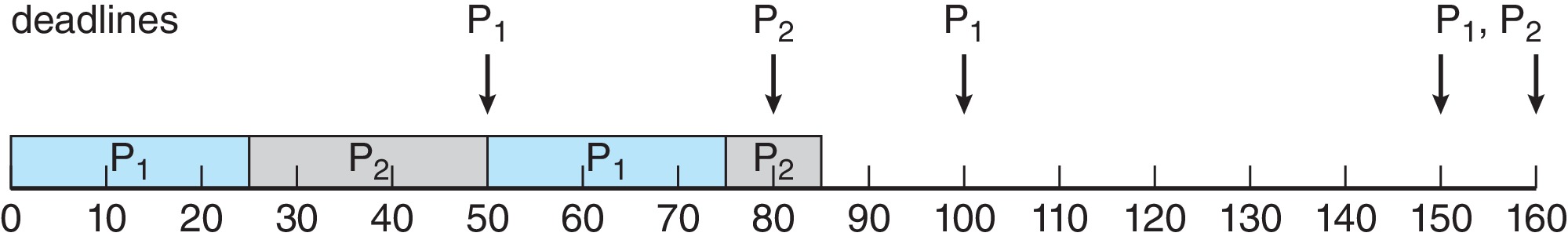
Figure 5.22: Rate-monotonic schedulingFigure 5.23: Missing deadlines with rate-monotonic scheduling
5.6.4 Earliest Deadline First Scheduling
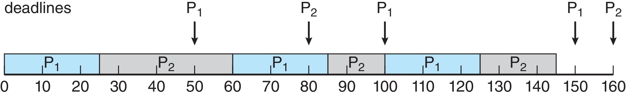
Figure 5.24: Earliest-deadline-first scheduling
EDF scheduling is an algorithm that minimizes maximum
lateness by giving priority to the process with
the earliest deadline. Relative priorities of processes
can change based on which future deadlines are currently
known.
EDF can perform better than Rate-monotonic scheduling, and
it does not require that processes be periodic, or that they
have fixed processing time t.
All that's required is that the process be able to 'announce'
its deadline to the scheduler when it becomes runnable.
5.6.5 Proportional Share Scheduling
Proportional share schedulers allocate shares of CPU time to
each member of a group of processes.
The scheduler admits a client process only if
the scheduler is able to allocate the number of shares
that the client requests.
5.6.6 POSIX Real-Time Scheduling
The POSIX standard provides extensions for real-time
computing.
Basically the scheduling possibilities are forms of
FIFO.
5.7 Operating System Examples
5.7.1 Example: Linux Scheduling
The Linux OS started out using a traditional Unix
scheduler, but in more current revisions began using
something called the Completely Fair Scheduler(CFS) due to
performance problems in systems with multiprocessors and/or large
numbers of processes.
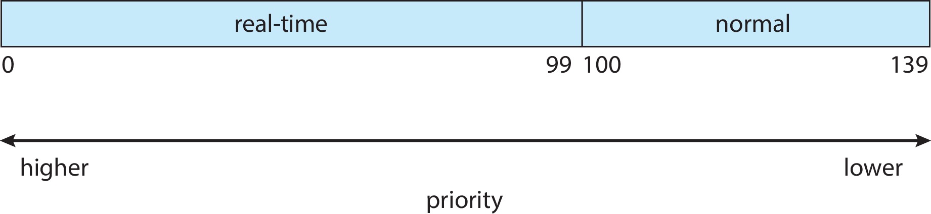
Standard Linux has two scheduling classes, "default"
and real-time. Each class has its own priority and
scheduling algorithm.
Figure 5.26: Scheduling priorities on a Linux system
CFS is the algorithm used for the default class.
CFS assigns a proportion of CPU time to each task,
according to its nice value, which is a
quantity traditionally used in unix-like systems as a
component of the process priority formula. We may think of
the nice value as a base priority.
The virtual runtime, or vruntime is the
overall CFS priority
of a process, calculated from its nice value (nv) and
its amount of recent (CPU) runtime (rrt). Lower values of either
nv or rrt correspond to higher CFS priority.
The CFS scheduler has a ready queue implemented as a
red-black tree. The scheduler caches the location of the
leftmost node, which represents a task with a minimum
value of vruntime - a maximum priority.
Linux supports real-time processing by implementing
POSIX Real-Time Scheduling (see section 5.6.6), and
by giving real-time processes higher priority than all
default-class processes.
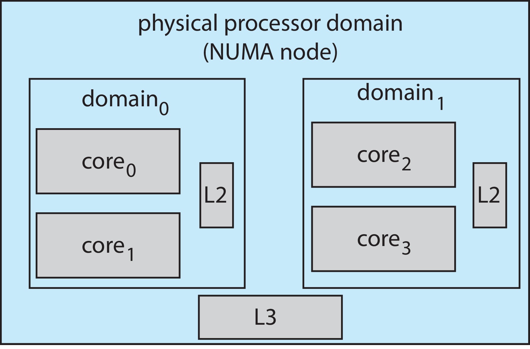
Figure 5.27: NUMA-aware load balancing with Linux CFS scheduler
The CFS scheduler also supports load balancing and
processor affinity. It tries to keep the total
load of the members of each ready queue
approximately equal. Load, roughly speaking,
is a measure of expected CPU usage. At the same
time, CFS tries to avoid migrating processes to cores
where they can no longer use current resources, like
L2 cache and on-chip memory.
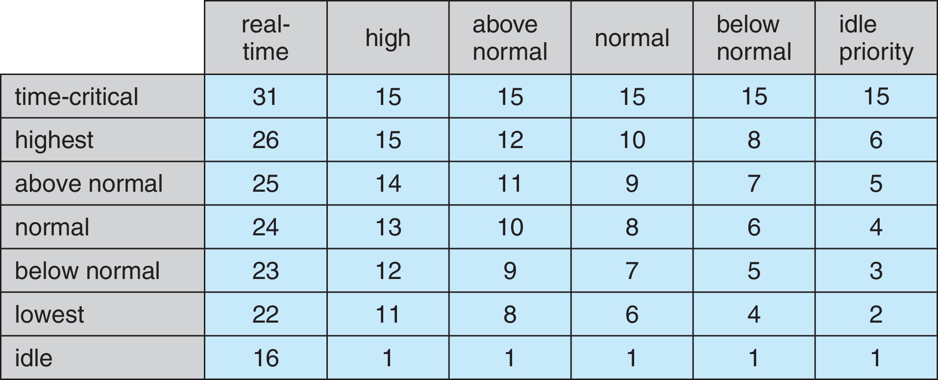
5.7.2 Example: Windows Scheduling
Windows has preemptive priority scheduling that gives
real-time processes higher priority than normal processes.
There are 32 levels of priority, each with its own queue. The scheduler
finds the non-empty queue with the highest priority and selects a thread there
for execution.
Figure 5.28: Windows Thread Priorities
The OS changes priorities of normal processes to help
improve response times and mitigate starvation
problems. Examples: lower the priority of a process that
uses its entire time slice, or raise the priority of a process
when it returns from waiting for I/O. Other examples: higher priority to threads
supporting the selected window, and longer time slices for threads
interacting with a user.
Windows 7 has user mode scheduling - a facility
that allows applications to create and schedule user-level
threads.
Windows supports processor affinity by defining
SMT sets of logical processors, and attempting
to keep each thread within its SMT set.
Windows also supports load balancing, by attempting
to make evenly-distributed initial assignments of
threads to processors.
5.7.3 Example: Solaris Scheduling
Solaris has six scheduling classes: time-sharing,
interactive, real time, system, fair share, and
fixed priority.
The Solaris time-sharing class is the default.
Solaris schedules the time-sharing class
with a multi-level feedback queue. Processes that have used
little CPU time lately get high priority. Lower priority
processes get larger time slices. The goal of that is to give
good response time to interactive, I/O-bound processes, while helping
CPU-bound processes to get good throughput.
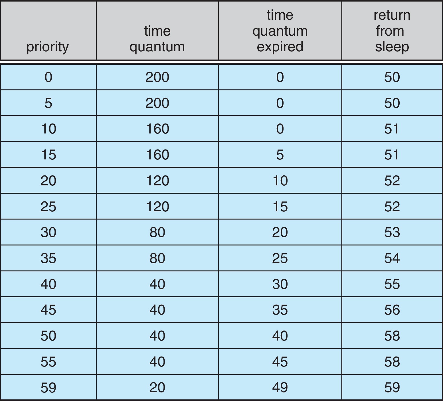
Figure 5.29: Solaris dispatch table for time-sharing and interactive threads
Solaris schedules the interactive class about the same way
as the time-sharing class, but it gives high priority to
windowing applications.
In scheduling the time-sharing and interactive classes,
Solaris gives smaller time slices to higher-priority
proceses. It also lowers the priority of processes
that use up their time slice, and it boosts priorities
of processes that have recently returned from sleep.
The scheduling algorithm for the time-sharing and
interactive classes is table-driven.
Processes in the real-time class have priority higher than
any other class.
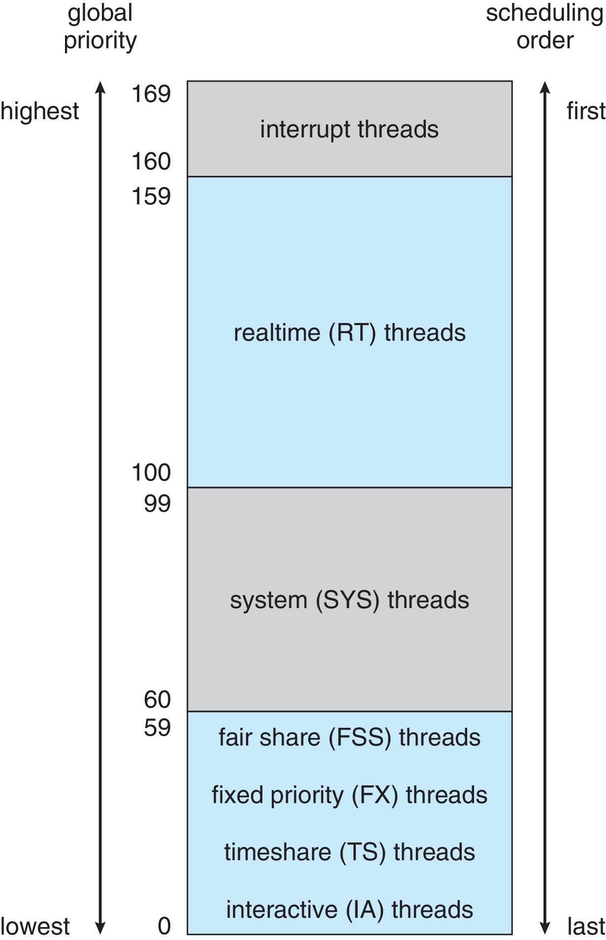
Solaris actually maps all the classes and priorities into a
single spectrum of global priorities, and the scheduler runs
the highest priority process in the ready queue. (It settles ties
by running the processes in RR style.)
5.8 Algorithm Evaluation (evaluation of scheduling algorithms)
How do we select CPU scheduling algorithms?
First we must choose the goals we want the scheduling algorithm to
achieve, such as response time of less than one second, or low variance
in wait time.
Next we need ways to evaluate algorithms to see if they will achieve the
chosen goals. That's what this section is about - various ways to evaluate scheduling algorithms.
Figure 5.30: Solaris scheduling
5.8.1 Evaluate scheduling algorithms using
Deterministic modeling
Calculate performance based on
specific test inputs -- this can be effective when trying to find a
good scheduling technique for a system that tends to run the same
kind of program over and over, often with very similar input from
run to run -- e.g. payroll processing, census calculations, and
weather prediction. This is not the style of most personal computer
users, but it is nevertheless not uncommon in business and
government.
5.8.2 Evaluate scheduling algorithms using
Queuing Models
Prepare by gathering system statistics.
distribution of CPU and I/O bursts
distribution of job arrival-time
Do queuing network analysis -- get figures for things like
average queue lengths and waiting times.
The mathematics can be difficult so often researchers make
simplifying assumptions.
Naturally the results may be "weaker" because of the
simplifying assumptions.
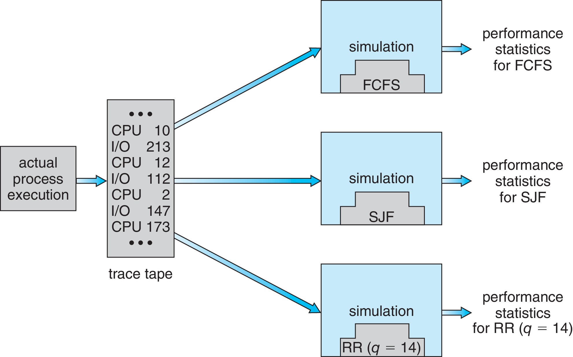
5.8.3 Evaluate scheduling algorithms using
Simulations
Represent major components and activities of the system with
software functions and data structures.
Use a variable to represent a clock and update system state
variables after each "tick."
Measure desired characteristics of the (simulation of the)
system.
Use random numbers and assumed distributions to produce inputs
to the system, or use traces from actual running systems.
Trace tapes have the advantage of making it possible to compare
different algorithms on the exact same inputs.
Random numbers and assumed distributions may not capture enough
information such as correlation in time between different kinds
of events.
Traces can take up a lot of space on secondary storage.
Simulations can be expensive to code and require long periods
of time to run.
Figure 5.31: Evaluation of CPU schedulers by simulation
5.8.4 Evaluate scheduling algorithms by
Implementation
Implement scheduling algorithms on an actual system
and measure their performance.
There are high costs of coding and system modification.
Inconvenience to users may be considerable.
User behavior may change in response to new scheduling
algorithm so the benefits of the algorithm may not
persist.
It may be useful to allow managers and users to "tune"
the scheduling policy of the running system, or to
provide API functions to modify priorities.
Solaris has a dispadmin command
for tuning the scheduling policy by changing
parameters of schedule classes. Java, POSIX,
and Windows APIs have functions for changing
the priority of a thread.